Automated Trading Course - Part 2: Strategy Design

This is the second part of the automated trading course, which will deal with how to write a profitable strategy. Some programming knowledge is required - for this, do the first part of the course if you haven’t already. It’s here: http://forums.babypips.com/expert-advisors-automated-trading/46881-automated-trading-course-part-1-programming.html

The second part will cover writing basic trading strategies, optimizing, walk forward analysis, portfolio strategies, and money management. It uses some new trading algorithms such as frequency filters. To avoid misunderstandings: It’s not a course about technical analysis. I won’t explain here moving averages or the like. It’s just about how to write a strategy based on a trading idea that you already have.

For the course you’ll need a program for running the script examples and testing the strategies. It’s called “Zorro” and you can download it for free from zorro-trader.com. Please also download the latest patch from the Zorro user forum, as the release had a bug in the chart display.

Two things to keep in mind:

► All strategies presented in this thread are meant for educational purposes. They are all profitable, but designed for simplicity, not for maximum profit or robustness. For really trading such a strategy, you would normally add entry filter rules for filtering out unprofitable trades. How to find and generate such rules with machine learning algorithms, such as Zorro’s perceptron or decision tree, might be covered in a future third part of the course. For really trading a strategy you normally also use a more sophisticated exit algorithm, realized with a trade management function. But that’s also stuff for a future part and we’ll keep it simple in this part of the course.

► I will post some backtest results here, but they can be slightly different to the results you’ll get when testing the scripts yourself. That’s because Zorro stores the current spread, commission, and rollover parameters for every asset when connecting to the broker. Because they change from time to time (and from broker to broker), backtest results also change. You can prevent this by setting Spread and other broker dependent parameters to a fixed value in the script, but keeping them in sync to the market gives a more realistic result.

Let’s start. The point of trading is knowing the moment when it’s good to buy, good to sell, or good to do nothing. Any trade strategy uses [B]market inefficiencies[/B] - deviations of the price curves from random data - for predicting future prices and finding the right buying and selling points. The most obvious way to make profits is going with the trend. Let’s have a little stage play in which trader Bob tries to explain his trade strategy to programmer Alice. Bob has just hired her to automatize his system:

Bob: I go with the trend. I buy long when prices start going up and I go short when they start going down.
Alice: And this works?
Bob: Sometimes. Depends on the market.
Alice: So you just buy long when today’s price bar is higher than the bars of the previous days?
Bob: Nah, one higher price bar alone won’t do. Prices wiggle a lot. Often the candles are all over the place. I look for the long term trend, like the trend of the last two months. I do that with a moving average.
Alice: Good. That shouldn’t be a problem to automatize.
Bob: Well, actually there is a problem. You see, a two month moving average lags at least one month behind the price. Often the trend is already over when the average finally bends up or down. You need to sort of look ahead of the moving average curve, if you get my meaning.
Alice: So you want to know when a two months trend changes, but you need to know it in far less time than two months?
Bob: You got it.
Alice: I could use a lowpass filter for getting the trend curve. Second order lowpass filters have almost no lag. Will that be ok for you?
Bob: I dunno what a second order lowpass filter is. But I trust you.
Alice: Good. So I buy when the trend curve changes its direction? For instance, when it starts to move up from a valley, or down from a peak?
Bob: You got it.
Alice: How do you exit trades?
Bob: When it’s the right time. Depends on the market.
Alice: I can exit a long position when entering a short one and vice versa. Does this make sense?
Bob: Yeah, that’s what I normally do when I’m not stopped out earlier.
Alice: Stopped out?
Bob: Sure. A trade must be stopped when it’s losing too much. We need a stop loss. Or do you want my whole account wiped from some bad trade?
Alice: Certainly not before I’m paid. At which price do you place the stop loss?
Bob: Not too far and not too tight. I don’t want to lose too much, but I also don’t want my trades stopped out all the time.
Alice: So let me guess: it depends on the market?
Bob: You got it.

Following the conversation, Alice wrote this trade strategy script for Bob, at a $5,000 fee:

function run()
{
  var *Price = series(price());
  var *Trend = series(LowPass(Price,1000));
  Stop = 2*ATR(100);

  if(valley(Trend))
    enterLong();
  else if(peak(Trend))
    enterShort();
}

When you did the first part of the course, you might recognize some familar structures, such as the [B]if[/B] statement, and some lines that look similar, but not quite like variable declarations. Tomorrow we’ll go thoroughly over this script, analyze what it does line by line, and then look in detail into the behavior and performance of this strategy.

This is how I see the if part.

If the trend function returns valley then execute the enterlong function, else if the trend function return peak… execute the entershort function

That’s correct. We’re now going to analyze the code. At first, we can see that the function is now named “[B]run[/B]” and not “[B]main[/B]”. “[B]run[/B]” is also a special function name, but while a main function runs only once, a [B]run[/B] function is called after every bar with the period and asset selected with the scrollbars. By default, the bar period is 60 minutes. So this function runs once per hour when Zorro trades.

At the begin we notice two strange lines that look similar to [B]var [/B]definitions:

[B]var *Price = series(price());
var *Trend = series(LowPass(Price,1000));[/B]

However unlike var definitions, they have an asterisk ‘[B]*[/B]’ before the name, and are set to the return value of a [B]series()[/B] function call. We define not a single variable here, but a whole [B]series[/B]. (C++ programmers might notice that we in fact define a [B]pointer[/B], but that needs not bother us now). A [B]series [/B]is a variable with a history - the series begins with the current variable value, then comes the value the variable had one bar before, then the value from two bars before and so on. This is mostly used for price curves and their derivatives. For instance, we could use a series to take the current price of an asset, compare it with the price from 1 bar before, and do some other things dependent on past prices. The series is the ideal construct for such price calculations.

The current value of a series can be used by adding a [B][0][/B] to the series name; for the value from one bar before add a [B][1][/B], for two bars before add a [B][2][/B] and so on. So, in Alice’s code [B]Price[0][/B] would be the current value of the [B]Price[/B] series, and [B]Price[1][/B] the value from 1 hour ago. Many trade platform languages - for instance, EasyLanguage - support series this way; usually indicator, statistics, and financial functions all use series instead of single variables. We’ll encounter series very often in trade scripts and will become familiar with them.

The [B]series()[/B] function can be used to convert a single variable to a series. The variable or value for filling the series is normally passed to that function. However, we’re not using a variable here, but the return value of a function call. [B]var *Price = series(price());[/B] means: define a [B]var [/B]series with the name “[B]Price[/B]” and fill it with the return value of the [B]price()[/B] function. We’ve learned in the last programming lesson how to ‘nest’ function calls this way, passing the return values of functions as parameters to other functions.

The [B]price()[/B] function returns the mean price of the selected asset at the current bar. There are also [B]priceOpen(), priceClose(), priceHigh()[/B] and [B]priceLow()[/B] functions that return the open, close, maximum and minimum price of the bar; however, the mean price is usually the best for trend trading strategies. It’s averaged over all prices inside the bar and thus generates a smoother price curve.

[B]var *Trend = series(LowPass(Price,1000));[/B]

The next line defines a series named “[B]Trend[/B]” and fills it with the return value from the [B]LowPass [/B]function. As you probably guessed, this function is the second order lowpass filter. Its parameters are the previously defined [B]Price[/B] series and a cutoff value, which Alice has set to 1000 bars. 1000 bars are about 2 months (1 week = 24*5 = 120 hours). Thus the lowpass filter attenuates all the wiggles and jaggies of the [B]Price [/B]series that are shorter than 2 months, but it does not affect the trend or long-term cycles above two months. It has a similar smoothing effect as a Moving Average function, but has the advantages of a better reproduction of the price curve and less lag. This means the return value of a lowpass filter function isn’t as delayed as the return value of a Moving Average function that is normally used for trend trading. The script can react faster on price changes, and thus generate better profit.

The next line places a stop loss limit:

[B]Stop = 2*ATR(100);[/B]

[B]Stop [/B]is a predefined variable that Zorro knows already, so we don’t have to define it. It’s the maximum allowed loss of the trade; the position is sold immediately when it lost more than the given value. The limit here is given by [B]2*ATR(100)[/B]. The [B]ATR [/B]function is a standard indicator. It returns the [B]Average Price Range[/B] - meaning the average height of a candle - within a certain number of bars, here the last 100 bars. So the position is sold when the loss exceeds two times the average candle height of the last 100 bars. By setting [B]Stop [/B]not at a fixed value, but at a value dependent on the fluctuation of the price, Alice adapts the stop loss to the market situation. When the price fluctuates a lot, higher losses are allowed. Otherwise trades would be stopped out too early when the price jumps down just for a moment.

A stop loss should be used in all trade strategies. It not only limits losses, it also allows Zorro’s trade engine to better calculate the risk per trade and generate a more accurate performance analysis.

The next lines are the core of Alice’s strategy:

if(valley(Trend))
  enterLong(); 
else if(peak(Trend)) 
  enterShort(); 

The [B]valley [/B]function is a [B]boolean[/B] function; it returns either true or false. It returns [B]true[/B] when the series just had a downwards peak. The [B]peak [/B]function returns [B]true[/B] when it just had an upwards peak. When the if(…) condition becomes true, a long or short trade with the selected asset is entered with a [B]enterLong [/B]or [B]enterShort [/B]command. If a trade was already open in the opposite direction, it is automatically closed. Note how we combined the [B]else [/B]of the first [B]if[/B] with a second [B]if[/B]; the second [B]if()[/B] statement is only executed when the first one was not.

Let’s have a look into an example trade triggered by this command:

The red line in the chart above is the [B]Trend [/B]series. You can see that it has a peak at the end of September 2008, so the [B]peak(Trend)[/B] function returned [B]true [/B]and the [B]enterShort [/B]function was called. The tiny green dot is the moment where a short trade was entered. The [B]Trend [/B]series continues downwards all the way until November 23, when a valley was reached. A long trade (not shown in this chart) was now entered and the short trade was automatically closed. The green line connects the entry and exit points of the trade. It was open almost 2 months, and made a profit of ~ 13 cents per unit, or 1300 pips.

In the next lesson we’ll learn how to backtest such a strategy and how to judge its profitability. There were a lot new concepts in this lesson, so please ask here if something is unclear or could be better explained.

Obviously, a strategy is worthless as long as you don’t know how it will perform. For this you need to run a backtest over at least 4 years, better 6 years. Start up Zorro, select the [Workshop4] script and the [EUR/USD] asset, leave the [Period] slider at 60 minutes, then click [Test]:

You might get a slightly different result when you downloaded the patch, as the default slippage was changed to better reflect worst case situations. By default, the simulation runs over the last 4 full years, i.e. from 2008 until 2011. The strategy achieves an annual profit of 94% - that’s the average profit per year divided by the sum of maximum drawdown and maximum margin. The monthly income (MI in the window) by this strategy is $115 - quite modest, but you traded with the minimum margin. $1465 capital is required for keeping a safe distance from a margin call. The figures are based on the investment of 1 lot per trade, usually equivalent to a $50 margin, the lowest possible trade size for a mini lot account.

Although 94% look a lot better than the usual 4% of a savings account, Alice is not too excited about the result. The Sharpe Ratio (SR) of 0.88 tells her that this result comes at a risk. The Sharpe ratio is the mean annual profit divided by its standard deviation. Sharpe ratios below 1 indicate that the gains fluctuate a lot - there might be years when the strategy achieves a lower profit, or even a loss. This is confirmed by the profit curve that Alice gets by clicking [Result]:

In the image that pops up in the chart viewer (if not, you need to install the patch from the Zorro forum), you can see a blue area, a black curve, and some green lines and red dots attached to the curve. The black curve is the price of the selected asset - the EUR/USD, i.e. the price of 1 EUR in US$. The price scale is on the left side of the chart. The green and red dots are winning and losing trades. The green lines connect the entry and exit point of a winning trade. You can see immediately that there are far more red than green dots - 88% of the trades are lost, only 12% are won. However, the long-term trades all have green lines. So we have a lot of small losses, but several large wins. This is the typical result of a trend following strategy.

The most interesting part of the chart is the blue curve that indicates our equity. We can see that it’s going up from zero in 2008 to $5500 (5.5K) at the end of 2011. This is a good thing. However the equity curve is quite shaky. The winning years are 2008 and 2010; in 2009 and 2011 we had a loss. This shaky behavior is reflected in the low Sharpe Ratio (SR) and the high Ulcer Index (UI). It would require strong nerves to trade such a strategy; there are long periods during which the strategy is losing money. Still, Alice thinks that this strategy is good enough for that lousy $5,000 programming fee, and Bob got what he wanted. We’ll learn in the next workshop how to write better strategies.

We can experiment a little by replacing the lowpass filter with other methods. When replaced with an traditional Exponential Moving Average (EMA) indicator, we had to use a shorter time period of 250 bars for getting about the same lag as a lowpass filter with 1000 bars. The second line in the code would then look like this:

var *Trend = series(EMA(Price,250));

and the system would be unprofitable, as an EMA with this short time period is too “jittery” for profitable trend trading with this method. Using lowpass filters instead of moving averages almost always improves the strategy performance, and often makes the difference between a winning and a losing system.

What have we learned so far?

► A strategy script contains a run function that is called once per bar.

► A series is a variable with a history.

► A lowpass filter removes the jaggies from a price curve without much lag penalty. It is superior to traditional moving averages.

► The valley and peak functions can be used to buy or sell at the turning points of a curve.

► A stop loss determines the trade risk.

Please post if something didn’t work or is unclear.

I forgot to mention - if someone wants to try this strategy in MT4 or other platforms, here’s the C source code of the LowPass, peak, and valley functions:

var smoothF(int period) { return 2./(period+1); }

var LowPass(var *Data,int Period)
{
	var* LP = series(*Data,3);
	var a = smoothF(Period);
	var a2 = a*a;
	return LP[0] = (a-0.25*a2)*Data[0]
		+ 0.5*a2*Data[1]
		- (a-0.75*a2)*Data[2]
		+ 2*(1.-a)*LP[1]
		- (1.-a)*(1.-a)*LP[2];
}

BOOL peak(var* a) { 
	return a[2] < a[1] && a[1] > a[0];
}

BOOL valley(var* a) {
	return a[2] > a[1] && a[1] < a[0];
}

In the next lesson we’ll look into how to optimize a strategy and use better test methods. Bob got a new trade idea:

Bob: Last month I ran into Warren Buffett and asked him for a trading advice. That’s what he said: ‘Be greedy when others are fearful’.
Alice: Interesting. And what does it mean?
Bob: He didn’t tell, but went away. But I think he wants me to go against the trend.
Alice: Isn’t that just the opposite of your last strategy?
Bob: You got it. I need you to automatize this. I now buy long when prices moved down very much, and go short when they moved up very much.
Alice: How much is very much?
Bob: Depends on the market.
Alice: I should have known.
Bob: Well, prices often move up and down in cycles. Problem is, cycles are sometimes not easy to see in the price curve. You must find the main price cycle and check if the price comes close to its top or bottom. Then you know the right moment to buy or sell.
Alice: I can use a frequency analysis function to find the dominant period of the price cycle.
Bob: If you say so.
Alice: Then I only need to find the top and bottom. I use the dominant period to control a highpass filter. This will cut off the trend and all cycles below the dominant period and give me a clean cycle curve.
Bob: Sounds good.
Alice: For finding how close the cycle is to its peaks, I must normalize the curve. For instance with a Fisher transformation. This has the advantage that the curve gets a Gaussian distribution. There are less extrema, and they are relatively sharp and well defined, so we won’t get too many false signals.
Bob: Sharp and well defined. I like that.
Alice: Of course it’s much more complicated than trend trading. This comes at a higher fee.
Bob: I like that less.
Alice: But I can run a Walk Forward Optimization as an extra.
Bob: Huh? Will that get me more profit?
Alice: Yes. So that you can afford me.

Alice went home and wrote this script (fee: $12,000):

function run()
{
  BarPeriod = 240; // 4 hour bars

// calculate the buy/sell signal 
  var *Price = series(price());
  var *DomPeriod = series(DominantPeriod(Price,30));
  var LowPeriod = LowPass(DomPeriod,500);
  var *HP = series(HighPass(Price,LowPeriod));
  var *Signal = series(Fisher(HP,500));
  var Threshold = 1.0;
  Stop = 2*ATR(100);

// buy and sell
  if(crossUnder(Signal,-Threshold)) 
    enterLong(); 
  else if(crossOver(Signal,Threshold))
    enterShort();

// plot signals and thresholds
  plot("DominantPeriod",LowPeriod,NEW,BLUE);
  plot("Signal",Signal[0],NEW,RED);
  plot("Threshold1",Threshold,0,BLACK);
  plot("Threshold2",-Threshold,0,BLACK);
  PlotWidth = 1000;
  PlotHeight1 = 300;
}

This system looks more complex than the simple trend trading system. Tomorrow we’ll go through the code and analyze it.

Couple of questions.
-The run function calls the whole code once per bar… does that mean if we are using 240 minute bar, the code is called once every 4 hours?
-Whats the difference between the BarPeriod and TimeFrame?
-I want to join the beta testers

  • Yes, every 4 hours.
  • It’s mostly the same, only the BarPeriod determines how often the script is executed, and there can be only one BarPeriod, but many TimeFrames in the same strategy. -> A better place for detail questions about Zorro parameters is the Zorro forum at Zorro Trading Automaton, this thread is for learning strategy writing only.
  • For joining the beta testers, register on the Zorro forum, then send a PM to the forum moderator, which happens to be me (jcl on that forum). I’ll then unlock the beta section for you.

Back to work. Alice has written the following script for a counter trend strategy:

function run()
{
  BarPeriod = 240; // 4 hour bars

// calculate the buy/sell signal 
  var *Price = series(price());
  var *DomPeriod = series(DominantPeriod(Price,30));
  var LowPeriod = LowPass(DomPeriod,500);
  var *HP = series(HighPass(Price,LowPeriod));
  var *Signal = series(Fisher(HP,500));
  var Threshold = 1.0;
  Stop = 2*ATR(100);

// buy and sell
  if(crossUnder(Signal,-Threshold)) 
    enterLong(); 
  else if(crossOver(Signal,Threshold))
    enterShort();

// plot signals and thresholds
  plot("DominantPeriod",LowPeriod,NEW,BLUE);
  plot("Signal",Signal[0],NEW,RED);
  plot("Threshold1",Threshold,0,BLACK);
  plot("Threshold2",-Threshold,0,BLACK);
  PlotWidth = 1000;
  PlotHeight1 = 300;
}

Counter trend trading is affected by market cycles and more sensitive to the bar period than trend trading. Bob has told Alice that bar periods that are in sync with the worldwide markets - such as 4 or 8 hours - are especially profitable with this type of trading. Therefore she has set the bar period to a fixed value of 4 hours, or 240 minutes:

BarPeriod = 240;

The counter trend trade rules are contained in the following lines that calculate the buy/sell signal:

var *Price = series(price());
var *DomPeriod = series(DominantPeriod(Price, 30));
var LowPeriod = LowPass(DomPeriod, 500);
var *HP = series(HighPass(Price, LowPeriod));
var *Signal = series(Fisher(HP, 500));

The first line sets up a price series just as in the last workshop. The next one calculates the dominant period. That’s the most significant cycle in a price curve which is normally a superposition of many cycles. If prices would oscillate up and down every two weeks, the dominant period would be 60 - that’s the length of two weeks, resp. 10 trade days, counted in 4-hour-bars. Alice uses the DominantPeriod() analysis function with a cutoff period of 30 bars for finding the main price oscillation cycle in the range below 100 bars. The result DomPeriod is a series of dominant periods.

Because the dominant period fluctuates a lot, the next line passes the series through a lowpass filter, just like the price curve of the last workshop. The result is stored in a variable (not a series, thus no ‘*’) LowPeriod that is the lowpass filtered dominant period of the current price curve.

In the next line, a highpass filter is fed with the price curve and its cutoff frequency is set to the dominant period. This removes the trend and all cycles that are lower than the dominant period from the price curve. The HighPass() function is similar to the LowPass function, it just does the opposite, and leaves only high frequencies, i.e. short cycles, in the price curve. The result is a modified price curve that consists mostly of the dominant cycle. It’s stored in a new series named HP (for HighPass).

Alice is not finished yet. The HP series is now compressed into a Gaussian distribution by applying the Fisher Transformation. This is an operation used to transform an arbitrary curve into a range where most values are in the middle - around 0 - and only few values are outside the +1…-1 range. For this transformation she calls the Fisher() function. It compresses the last 500 bars from the HP series into the Gaussian distributed Signal series. This method of trading with highpass filters, cycle detectors, and Fisher transform was developed by John Ehlers, an engineer who used signal processing methods for trading.

The next two lines define a new variable Threshold with a value of 1.0, and place a stop loss at an adaptive distance from the price, just as in Alice’s trend trading script from some lessons ago. The ATR function is again used to determine the stop loss.

var Threshold = 1.0;
Stop = 2*ATR(100);

Now that the preparation is done, we can start trading:

if(crossUnder(Signal, -Threshold))
enterLong();
else if(crossOver(Signal, Threshold))
enterShort();

When the Signal curve cosses the negative threshold from above - meaning when Signal falls below -1 - the price is supposedly at the bottom of the dominant cycle, so we expect the price to rise and buy long. When the threshold is crossed from below - meaning Signal rises above 1 - the price is at a peak and we buy short. This is just the opposite of what we did in trend trading. For identifying the threshold crossing we’re using the crossOver() and crossUnder() functions.

  • Obviously, these trade rules are somewhat more complicated than the simple lowpass function of the previous lesson. So Alice needs to see how the various series look, for checking if everything works as supposed. The next line (at the end of the script)

plot(“DominantPeriod”, LowPeriod, NEW, BLUE);

generates a plot of the LowPeriod variable in a NEW chart window with color BLUE. We can use this function to plot anything into the chart, either in the main chart with the price and equity curve, or below the main chart in a new window. The Signal curve and the upper and lower Threshold are plotted in another new chart window:

plot(“Signal”, Signal[0], NEW, RED);
plot(“Threshold1”, Threshold, 0, BLACK);
plot(“Threshold2”, -Threshold, 0, BLACK);

The first statement plots the Signal[0] value as a red curve (as we remember, adding a [0] to a series name gives its most recent value). The next two statements plot the positive and negative Threshold with two black lines in the same chart window. Note that the plot function always expects a value, not a series - that’s why we needed to add the [0] to the Signal name.

PlotWidth = 1000;
PlotHeight1 = 300;

This just sets the width and height of the chart window. Below is the resulting chart. Load the script workshop5_1 and make sure that EUR/USD is selected. Click [Test], then click [Result]:

The blue curve in the middle window is the plot of LowPeriod. It moves mostly between 25 and 40 bars, corresponding to a 4…7 days dominant cycle. The bottom window shows the Signal series. The black lines are the thresholds that trigger buy and sell signals when Signal crosses over or under them. Plotting variables and series in the chart greatly helps to understand and improve the trade rules. For examining a part of the chart in details, the StartDate and NumDays variables can be used to limit the number of bars to plot and ‘zoom into’ a part of the chart.

We can see that the script generates 139% annual return. This is already better than the simple trend trading script from the last workshop; but the equity curve is still not satisfying. Alice has to do more for her fee and improve this strategy further. We’ll do that tomorrow.

Today we’ll learn how to improve strategy’s performance with optimization. That basically means that some essential strategy parameters are optimized to achieve the maximum profit for a certain bar period, asset, and market situation. That’s why all better trade platforms have an optimizer, usually with an extra window or program outside the script. With Zorro, the script controls anything, and thus also determines which parameters are optimized in which way.

Alice’s has added some commands to the strategy for parameter optimization (select Workshop5_2):

function run()
{
  set(PARAMETERS);  // generate and use optimized parameters
  BarPeriod = 240;  // 4 hour bars
  LookBack = 500;   // maximum time period

// calculate the buy/sell signal with optimized parameters
  var *Price = series(price());
  var Threshold = optimize(1.0,0.5,2,0.1);
  var *DomPeriod = series(DominantPeriod(Price,30));
  var LowPeriod = LowPass(DomPeriod,500);
  var *HP = series(HighPass(Price,LowPeriod*optimize(1,0.5,2)));
  var *Signal = series(Fisher(HP,500));
  Stop = optimize(2,1,10) * ATR(100);

// buy and sell
  if(crossUnder(Signal,-Threshold))
    enterLong(); 
  else if(crossOver(Signal,Threshold))
    enterShort();

  PlotWidth = 1000;
  PlotHeight1 = 300;
}

Parameter optimization requires some additional settings at the begin of the script:

set(PARAMETERS);
BarPeriod = 240;
LookBack = 500;

PARAMETERS is a “switch” that, when set, tells Zorro to generate and use optimized parameters. LookBack must be set to the ‘worst case’ lookback time of the strategy. The lookback time is required by the strategy for calculating its initial values before it can start trading. It’s usually identical to the maximum time period of functions such as HighPass() or Fisher(). If the lookback time depends on an optimized parameter, Zorro can not know it in advance; so we should make it a habit to set it directly through the LookBack variable when we optimize a strategy. In this case we set it at 500 bars to be on the safe side.

The signal calculation algorithm now also looks a little different:

var Threshold = optimize(1, 0.5, 2);
var DomPeriod = DominantPeriod(Price, 30);
var LowPeriod = LowPass(DomPeriod, 500);
var *HP = series(HighPass(Price, LowPeriod * optimize(1, 0.5, 2)));
var *Signal = series(Fisher(HP, 500));
Stop = optimize(2, 1, 10) * ATR(100);

Some parameters have now been replaced by optimize function calls. We also notice that the line with the Threshold variable has now moved to the begin of the code. This is because more important parameters should be optimized first, and the most important is Threshold which determines the sensitivity of the strategy and has the largest influence on its profit. It is now set to the return value of the optimize function. optimize is called with 3 numbers; the first is the parameter default value, which is 1 - just the value that Threshold had before. The next two numbers, 0.5 and 2, are the parameter range, i.e. the lower and upper limit of the Threshold variable. So Threshold can now have any value from 0.5 to 2. During the optimization process, Zorro will try to find the best value within this range.

Alice has selected two more parameters to be replaced by optimize calls: a factor for the HighPass time period, and a factor for the stop loss distance. The default values are just the values used in the first version of the counter trading script. Theoretically, there could be even more parameters to optimize - for instance the DominantPeriod cutoff value, or the number of bars for the ATR function. But the more parameters we have, and the larger their range is, the higher is the danger of overfitting the strategy. Overfitted strategies perform well in the simulation, but poor in real trading. Therefore only few essential parameters should be optimized, and only within reasonable parameter ranges.

For training the strategy, click [Train] and observe what the optimize calls do. During the training phase, which can take about one minute depending on the PC speed, you’ll see the following charts pop up:


Parameter 1 (Threshold)


Parameter 2 (LowPeriod factor)


Parameter 3 (Stop factor)

The parameter charts show how the parameter values affect the performance of the strategy. The red bars are the profit factor of the training period - that is the total win divided by the total loss. The dark blue bars are the number of losing trades and the light blue bars are the number of winning trades. We can see that Threshold has two profit maxima at 1.10 and 1.50; the LowPeriod factor has a maximum slightly above 1. The Stop factor - the 3rd parameter - has a maximum at about 7. We can also see that a distant stop, although it increases the risk, also increases the number of profitable trades, the ‘accuracy’ of the strategy.

The 3 optimized parameters are stored in the file Data/Workshop5_2_EURUSD.par. Different parameter sets could be generated for other assets. A click on [Test], then on [Result] displays the equity chart of the optimized strategy:

We can see how training has improved the script. The annual return now exceeds 200%, meaning that the invested capital doubles every 6 months. The new Sharpe Ratio is well above 1, meaning that this strategy is really tradable. Or is it? Well, in fact it’s too good to be true. If Alice would deliver the strategy with this test result, she would have made a severe mistake and Bob would probably not get as rich as expected. What’s the problem?

Alice has used the price data from the last 4 years for optimizing the parameters, and has used the same price data for testing the result. This always generates a too optimistic result due to curve fitting bias. It also has a second problem. In 4 years, markets change and trading strategies can become unprofitable. It is not recommended to trade an optimized strategy unchanged for 4 years. Normally the strategy parameters should be re-optimized in regular intervals for adapting them to the current market situation. Zorro can do that automatically while life trading, but how can we simulate this in a test and get some realistic prediction of the real trading behavior?

The answer is Walk-Forward Optimization. That will be our topic for tomorrow.

Please post here if there are questions or something is unclear.

ok got it your a TA and not a trader i can see why you have currupted all my threads…that are intended to help traders.

If a strategy fails in a walk forward optimization, it will also fail in real trading, even if it performed well in a backtest. For this reason, walk forward optimization is the most important process when developing a strategy or EA - and this lesson today is the most important one for learning strategy development.

Contrary to its name, Walk Forward Optimization (WFO) is not really an optimization. It’s a test method that tests not only the strategy algorithm, but also its parameter ranges and its optimization settings. For this Alice just adds two lines at the begin of the script (Workshop5_3):

[B]NumWFOCycles = 8;
NumBarCycles = 4;[/B]

The first line activates WFO with a data frame that is shifted in 8 cycles over the simulation period. The frame consists of a training period and a subsequent test, as in the figure below:

The training period generates the parameters that are then tested in the subsequent test period. This makes sure that every test uses “unseen” price data that was not used for optimizing its parameters - just as it would happen in real trading. The data frame is then shifted over the simulation period for verifiying how the strategy would fare when started at different times.

However, there’s a problem. Obviously WFO uses less price data than an optimization over the full simulation period. The less trades are simulated in the optimization and test process, the less accurate is the result. For getting more trades per WFO cycle, Alice could use a longer cycle period. Problem is that the markets change over time, so a price curve from 2009 likely requires different strategy parameters than a price curve from 2011. When using more than about one or two year’s price data for a WFO cycle, the data covers too different market periods, which often makes optimization ineffective. The result is then worse and not better.

Therefore, the challenge is not using more data, but getting more trades out of the same data. Because historic price data is available in a much higher resolution than the bar period, a method called ‘[B]Oversampling[/B]’ can be used for increasing the number of trades. The simulation is repeated several times. Every time the bars are resampled with a different offset into the price data. This generates a set of curves with slightly different bars that trigger different trades in every curve, while at the same time maintaining the trends, periodic behavior, and other characteristics of the original price curve.

For this Alice has set the [B]NumBarCycles[/B] variable to [B]4[/B]. This runs the simulation 4 times with resampled bars, and calculates the performance and equity curve from the average of the 4 simulation cycles. Oversampling can remarkably increase the quality of the optimization process, as well as the accuracy of the test result. Of course, oversampling has a limit - we’re still using the original prices after all, only the bars are built in a different way. The method does not much improve strategies that are based on very smoothed trend curves, such as for the crossing of two very long-period moving averages. But it works well for strategies that use the high-frequency part of a price curve.

After loading the Workshop5_3 script, click [Train]. Training now takes a few minutes because a full optimization is performed for every cycle, and the process is repeated 4 times with oversampling. The optimized parameters are now stored in a different parameter file for every WFO cycle. They are used when you click [Test] after the optimization process. Again, depending on the current price data your result might look slightly different:

Click [Result] for getting the chart below:

We can see that the test now only covers 2 years; no testing happens in 2008 and 2009 as they are used up for the lookback and training periods. Still, the strategy stays profitable with WFO optimization. The Sharpe Ratio is even a little better because parameter values now follow the market more closely. The strategy achieves a Profit Factor of more than 4, meaning that the average gain is four times the average loss. This is an excellent result. At least in theory…

When life trading this strategy, its parameters must be regularly re-calculated and adapted to the current market situation, just as in the WFO process. For this, Alice has added the following lines to the script:

if(ReTrain) {
  UpdateDays = 30; 
  SelectWFO = -1; 
}

[B]ReTrain[/B] is nonzero when the [Train] button is clicked during life trading. [B]UpdateDays [/B]is the time period for loading new price data from the broker’s server; in this case new price data is loaded when the price data to be used for optimization is older than 30 days. [B]SelectWFO [/B]tells Zorro not to optimize the whole simulation period, but only a certain WFO cycle; in this case, the last cycle that contains the new price data.

Clicking [Train] every couple of months will continue the WFO process during trading, and makes the strategy independent of external parameter settings - we have essentially a ‘parameter-free’ strategy. Can we really expect 215% annual return and $362 average monthly income when we let Zorro trade it this way? Maybe in the long run, but the prediction error (Error in the message window) is over 60% - that means the profit after 2 years can be anything between $3000 and $15000. And we have still long periods, as in the first part of 2011, with no profit. Tomorrow we’ll learn how to make strategy returns more steady and reliable so that Bob can really derive a regular income from them.

What have we learned so far?

► The [B]DominantPeriod [/B]function returns the main cycle of the price curve. It can be used to control filters or indicators.

► The [B]HighPass [/B]filter removes the trend from a price curve.

► The [B]Fisher transform[/B] compresses a curve to a Gaussian distributed range.

► The [B]plot [/B]function displays the curves of signals and indicators.

► The [B]crossOver [/B]and [B]crossUnder [/B]functions detect the crossing of a curve with a threshold or with another curve.

► [B]Optimize [/B]parameters for improving a strategy.

► [B]Walk Forward Optimization[/B] simulates trading under realistic conditions for parameter-free strategies.

► [B]Oversampling [/B]improves the optimizing quality and and the test accuracy.

► WFO optimized strategies should be [B]re-trained[/B] in regular intervals.

Tomorrow we’ll start with the last lesson about portfolio trading. You’ll also learn that money management is very different to the “trade only 1% of your account” newbie wisdom.

Bob: I got it! This is it!
Alice: Bob! Why are you running naked through the streets?
Bob: Huh? Oh, I was just sitting in my bathtub when I suddenly got this brilliant idea. I need you to program it immediately. This will solve all my trading problems!
Alice: Problems? I thought you were already getting rich by automated trading?
Bob: It started well, but then went all wrong. You know, from all the systems you programmed for me, the counter trend system worked best.
Alice: I figured that.
Bob: And from all assets, I found it had the most profit with the EUR/USD. So I invested all my money in that system trading with EUR/USD.
Alice: Oh no!
Bob: Yes! And it worked like a champ! My account went up from $100,000 to $350,000 in six months. I naturally began to think about what do do with all that money, and had already ordered a Porsche and a golden bathtub.
Alice: Naturally.
Bob: But then all of the sudden, your system started losing money. My account went down and down and didn’t stop going down.
Alice: How much?
Bob: It lost almost $150,000 in a single month. I’m now back at $210,000, and it’s staying there since weeks.
Alice: This is a drawdown. Profitable strategies have always drawdowns - look at the equity curves. You should worry if you have no drawdown, because that wouldn’t be normal. You can’t do much anyway. Just sit it out.
Bob: I don’t have the nerve for that. Every morning I’m looking at the PC and my account is either going down, or not going up!
Alice: Put a blanket over your PC.
Bob: I got a much better idea. That’s why I was on the way to you. What if the system traded with many assets at the same time?
Alice: Yes, that could increase the Sharpe Ratio when the assets are not correlated.
Bob: I dunno what you mean with that. But I know that when EUR/USD is moving sidewards, chances are that a different pair, like USD/CHF, is just trending or cycling. So I lose with one but win with the other, if you get my meaning. And I can do this with many more assets.
Alice: Yes. That’s portfolio trading.
Bob: And can’t you also combine your systems into one? I mean a super system that goes with the trend and against the trend at the same time? So I win when assets are trending and I also win when assets are cycling? Meaning I win all the time?
Alice: You won’t win all the time, because the equity curves of strategies are often more or less correlated. But it will certainly reduce your drawdowns and improve the annual profit.
Bob: Well, then program this. I’ll sell my Porsche and pay you well.
Alice: I’ll start at once. Now better go home and put some clothes on.

Bob has given Alice the task to write a script that trades with several assets simultaneously, and uses both trend and counter-trend strategy algorithms. This is her first version (Workshop6_1 script, agreed fee: $28,000):

// Trend trading function from Workshop 4
function tradeTrend()
{
  var *Price = series(price());
  var *Trend = series(LowPass(Price,optimize(250,100,1000)));
  Stop = optimize(2,1,10) * ATR(100);
  
  if(valley(Trend))
    enterLong();
  else if(peak(Trend))
    enterShort();
}

// Counter trend trading function from Workshop 5
function tradeCounterTrend()
{
  var Threshold = optimize(1.0,0.5,2,0.1);
  var *DomPeriod = series(DominantPeriod(Price,30));
  var LowPeriod = LowPass(DomPeriod,500);
  var *HP = series(HighPass(Price,LowPeriod*optimize(1,0.5,2)));
  var *Signal = series(Fisher(HP,500));
  Stop = optimize(2,1,10) * ATR(100);

  if(crossUnder(Signal,-Threshold))
    enterLong();
  else if(crossOver(Signal,Threshold))
    enterShort();
}

function run()
{
  set(PARAMETERS);   // use optimized parameters factors
  BarPeriod = 240;   // 4 hour bars
  LookBack = 500;    
  NumWFOCycles = 8;  // activate WFO, 8 cycles
  NumBarCycles = 4;  // 4 times oversampling
 
  if(ReTrain) {
    SelectWFO = -1;   // when re-optimizing, select the last cycle only
    UpdateDays = 30;	// reload new price data from the server every 30 days
  }

// double portfolio loop
  while(asset(loop("EUR/USD","USD/CHF")))
  while(algo(loop("TRND","CNTR")))
  {
    if(Algo == "TRND") 
      tradeTrend();
    else if(Algo == "CNTR") 
      tradeCounterTrend();
  }
}

The two first functions of this script should look familiar. Tomorrow we’ll check out what the rest is doing.

[QUOTE=jcl365;399054]

Bob has given Alice the task to write a script that trades with several assets simultaneously, and uses both trend and counter-trend strategy algorithms. This is her first version (Workshop6_1 script, agreed fee: $28,000):

It sounds like writing a script is more profitable than actually trading it :)). But seriously thanks for very interesting tread, i code my EA’s in MQL4, but this C looks a lot less complicated. i definitely have to learn it.

Thanks! Of course, the price of a script depends on its quality ;).

Back to the script. The strategy is now divided into 3 different functions: tradeTrend() for trend trading, tradeCounterTrend() for counter trend trading, and the run() function that sets up the parameters, selects the assets, and calls the two trade functions.

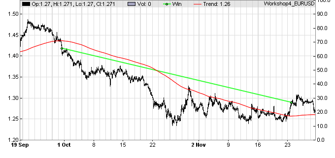
The tradeTrend() function uses the same trade algorithm as at in the first script of this course, only this time the LowPass time period and the stop loss value are optimized. Note that the time period parameter has a different value here, as one bar is now 240 minutes, compared to 60 minutes in the first version of the strategy. So the parameter must be smaller by a factor 4 for getting the same time period.

The tradeCounterTrend() function and the begin of the run() function are similar to the final version of the counter trend trading script. However, the core of the strategy looks very different:

while(asset(loop("EUR/USD","USD/CHF")))
while(algo(loop("TRND","CNTR")))
{
  if(Algo == "TRND")
    tradeTrend();
  else if(Algo == "CNTR")
    tradeCounterTrend();
}

We have two ‘nested’ while loops, each with two nested functions. Let’s untangle them from the inside out:

loop(“EUR/USD”,“USD/CHF”)

The loop function takes a number of arguments, and returns one of them every time it is called. On the first call it returns the first parameter, which is the string “EUR/USD”. We have learned in the first programming lesson that a string is a variable that contains text instead of numbers. Strings can be passed to functions and returned from functions just as numerical variables. If the loop function in the above line is called the next time, it returns “USD/CHF”. And on all futher calls it returns 0, as there are no further arguments.

asset(loop(“EUR/USD”,“USD/CHF”))

The strings returned by the loop function are now used as arguments to the asset function. This function selects the asset to trade with in the following part of the code - just as it it had been choosen with the [Asset] scrollbox. The string passed to asset must correspond to an asset subscribed with the broker. If asset is called with 0 instead of a string, it does nothing and returns 0. Otherwise it returns a nonzero value. This can be taken advantage of in a while loop:

while(asset(loop(“EUR/USD”,“USD/CHF”)))

This loop is repeated as long as the while argument, which is the return value of the asset function, is nonzero (a nonzero comparison result is equivalent to ‘true’). And asset returns nonzero when the loop function returns nonzero. Thus, the while loop is repeated exactly two times, once with “EUR/USD” and once with “USD/CHF” as the selected asset. If Alice had wanted to trade the same strategy with more assets - for instance, also with commodities or stock indices - she only needed to add more arguments to the loop function, like this:

while(asset(loop(“EUR/USD”,“USD/CHF”,“USD/JPY”,“GBP/USD”,“XAU/USD”,“USOil”,“SPX500”,“NAS100”,…)))

and the rest of the code would remain the same. However, Alice does not only want to trade with several assets, she also wants to trade different algorithms. For this, nested inside the first while loop is another while loop:

while(algo(loop(“TRND”,“CNTR”)))

The algo function basically copies the argument string into the predefined Algo string variable that is used for identifying a trade algorithm in the performance statistics. It also returns 0 when it gets 0, so it can be used to control the second while loop, just as the asset function in the first while loop. Thus, for every repetition of the first loop, the second loop repeats 2 times, first with “TRND” and then with “CNTR”. As these strings are now stored in the Algo variable, Alice uses them for calling the trade function in the inner code of the double loop:

if(Algo == "TRND")
  tradeTrend();
else if(Algo == "CNTR")
  tradeCounterTrend();

As we see, a string variable can be compared to a string constant just as if we would compare a numeric variable to a numeric constant. Due to the two nested loops, this inner code is now run four times per run() call:

  • First with “EUR/USD” and “TRND”

  • Then with “EUR/USD” and “CNTR”

  • Then with “USD/CHF” and “TRND”

  • And finally with “USD/CHF” and “CNTR”

If Alice had instead entered 10 assets and 5 algorithm strings in the loop arguments, the inner code would be run fifty (10*5) times every bar.

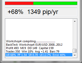
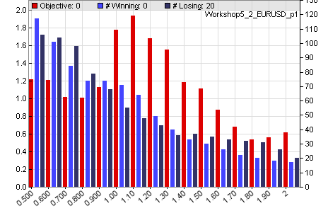
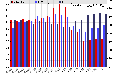
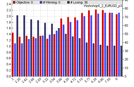
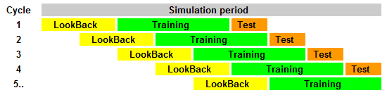
Now it’s time to [Train] the strategy. Because we have now four components - asset/algorithm combinations - the training process now takes four times longer than with the last script. As soon as it’s finished, let’s examine the resulting parameters. Use the SED editor to open the Workshop6_1_1.par file in the Data folder. This file contains the optimized parameters from the first WFO cycle. It should look like this:

EUR/USD:TRND 420 1.62 => 1.896
EUR/USD:CNTR 0.998 0.976 6.15 => 2.605
USD/CHF:TRND 673 1.34 => 1.343
USD/CHF:CNTR 1.20 0.812 2.38 => 1.980

As we can see, every line begins with the identifier for the asset and algorithm; then follows the list of parameters. This allows Zorro to load the correct parameters at every asset() and algo() call. We can see that the tradeTrend() function uses 2 parameters and the tradeCounterTrend() function uses 3 parameters, and their optimal values are slightly different for the “EUR/USD” and the “USD/CHF” assets. The last number behind the “=>” is not a parameter, but the result of the objective function for the final optimization; it can be ignored.

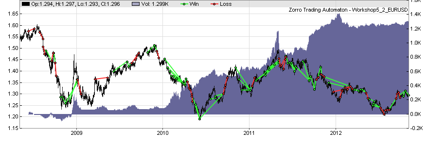
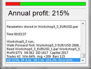
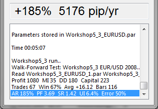
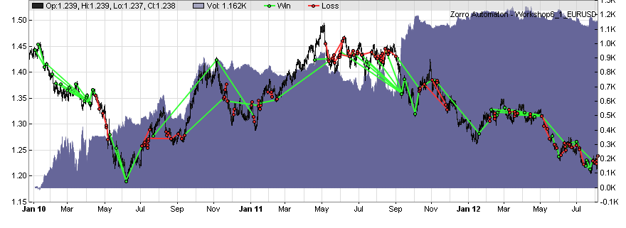
Finally, let’s have a look at the performance of this portfolio strategy. Click [Test], then click [Result].

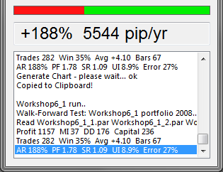
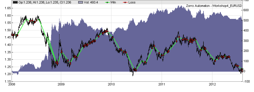
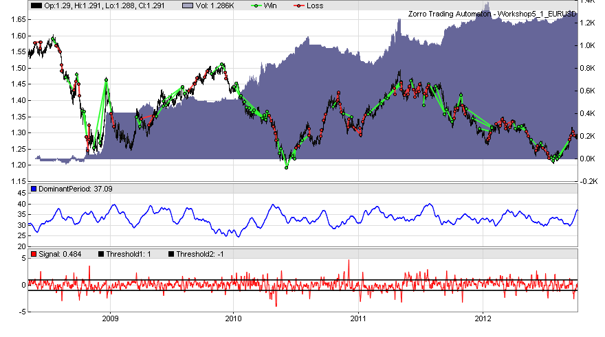
You can see in the chart that now two different strategies are traded simulaneously. The long green lines are from trend trading where positions are hold a relatively long time, the shorter lines are from counter-trend trading. The combined strategy does both at the same time.

Now look at the end of the performance sheet that popped up when clicking [Result]. You can see how the single components were performing during the test:

Trade details       OptF  ProF  Win/Loss  Cycles
 
EUR/USD total       .048  2.42   37/57    /XXXXXX
USD/CHF total       .059  1.55   27/62    XXX\XX/
 
CNTR total          .052  2.14   48/51    XXXXX/X
TRND total          .055  1.57   16/68    XXXXXXX
 
EUR/USD:CNTR:L      .025  1.54    7/9     ///\\/\
EUR/USD:CNTR:S      .086  6.34   20/6     //././/
EUR/USD:TRND:L      .034  1.43    7/18    ..\//\\
EUR/USD:TRND:S      .000  0.80    3/24    .\\\\\/
USD/CHF:CNTR:L      .000  0.97   12/21    /\\\\//
USD/CHF:CNTR:S      .044  1.88    9/15    \\/\//.
USD/CHF:TRND:L      .088  2.20    3/13    //\\.\/
USD/CHF:TRND:S      .044  2.58    3/13    \\/\./.

The performance is listed separately for long (":L") and short (":S") trades. We can see that the components performed very different: The best performer is EUR/USD:CNTR with a profit factor (ProF) 1.54 for long, and 6.34 for short trades - that’s the algorithm from the last workshop. The worst performer is EUR/USD trend trading; however with the USD/CHF asset, trend trading performs much better.

Wouldn’t it be wise to invest more money in the more profitable components, less money in the less profitable, and no money at all in the components that turned out unprofitable in the test? That’s called “money management” and will be the topic of the next lesson.

if anyone wants to make a robot i know as a self full time trader the simple entry exit points and what price has to equel and so on…then lets colabarate

Dennis how do u mean?

i think it would be worthwile if there was a automated trading system that could buy and sell my rules. Do not know if its possible, I am not very tech to be honest unless its about fixing engines.

I know what i would want a automated trade system to do but i would not know how to program it to do it.

I am purely a manual trader with clear charts apart from MA and fibs and trendlines

example rule: if current candle closes below 20 sma and the candle is within 40 pips of the 200 SMA sell to the touch of the 200 SMA , SL 2 pips aboove the 20 SMA.

thats sort of thing am I in the right place for this? really I am so low tech on Computing

That’s what the thread covers, automated trading. We are learning here…if you take the time to learn, I am sure Jcl will be ready to help if you do some of the work yourself