So I’ve starting using MT5 this time around. And I’ve gone downloaded data into excel as a .csv file.
When I open the file I see the following text.
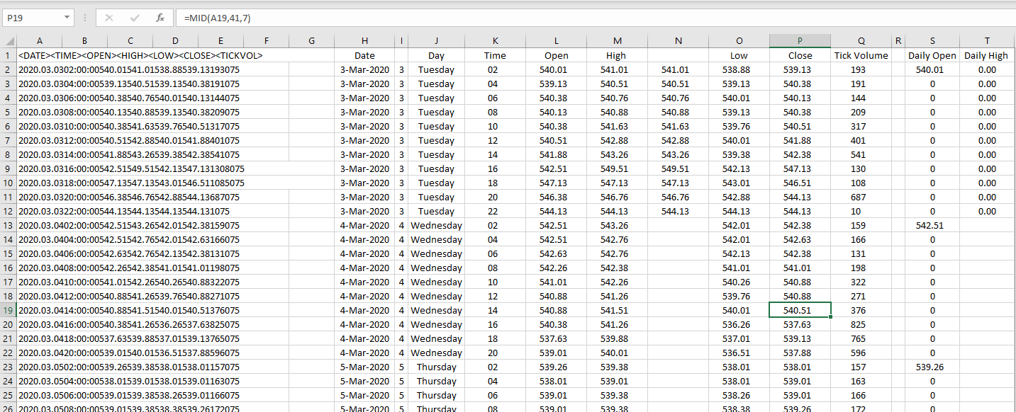
“2020.03.03 02:00:00 540.01 541.01 538.88 539.13 193 0 75”
No biggie. I simply use “=MID()” to extract the data (date, time, open, high, low, close, volume) into columns for analysis.
However when I then use a function like “=MAX()” to analysis each array (column), (this case maximum value) it returns zero.
I like to think I’m pretty good in excel but this has got me stumped, any help???
.csv files have field (column) separators by default. Usually they are commas (csv = comma separated value) but it’s not unusual to find colons, semi-colons, pipe ( | ), tabs and even space characters. Excel and similar spreadsheet programs have the ability to distinguish these separators and split them into separate columns using the “Text to Columns” feature.
Can’t say for certain what’s going on with the MAX formula till you show the syntax. The formula bar in the scr shot shows the syntax for the MID formula in cell P19.
The gif shows me working on an MT5 dump. There are two parts. The first part shows the steps to split the data into each column with steps as folls:
- Validating delimiter/separator value in a text editor and determining it was a tab. Not a necessary step 90%+ of the time. But useful to know in case you have a bad data file with messed up delimiters.
- Open CSV in Excel (I use an WPS Sheet, which have similar layouts)
- Navigate to Data > Text to Columns
- Specify “Delimited” as data type.
- Ensure “Tab” selected as delimiter in step 2.
- Step 3 is and important step. I specify the date format in the CSV so excel recognizes it and translates it properly considering your regional settings. This can cause havoc with date based data if you’re not careful.
- Hit finish and wait a bit while it finishes processing 75K+ records.
In the second part I use a pivot table to aggregate the data by month and extract the Max Close values. The formula option is long and convoluted for the same solution (if it’s even possible; I didn’t think too much about it). Steps:
- Create two new columns and extract YEAR and MONTH values from the column
- Select data range (select all or CTRL+A in this case)
- Navigate and click Data > Pivot Table
- Validate range in step 1and select pivot table display in same worksheet or new one. Click “OK”
- Select and drag newly defined Year and Month columns to “ROWS”
- Select and drag CLOSE to values
- Open context menu for default “Sum of CLOSE” value and select “Value field settings”
- Select “Max” and click OK.